Pairs Trading
Pairs trading is a form of mean-reversion that has a distinct advantage of always being hedged against market movements. It is generally a high alpha strategy when backed up by some rigorous statistics. The stratey is based on mathematical analysis.
The prinicple is as follows. Let’s say you have a pair of securities X and Y that have some underlying economic link. An example might be two companies that manufacture the same product, or two companies in one supply chain. If we can model this economic link with a mathematical model, we can make trades on it.
Assumption
- Economical ties
- Mean Reversion
General Process
-
Cluster Stock Universe
-
Find pairs of stocks with conintegration
-
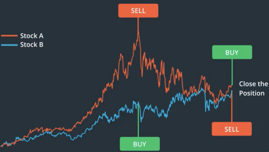
Buy low, sell high
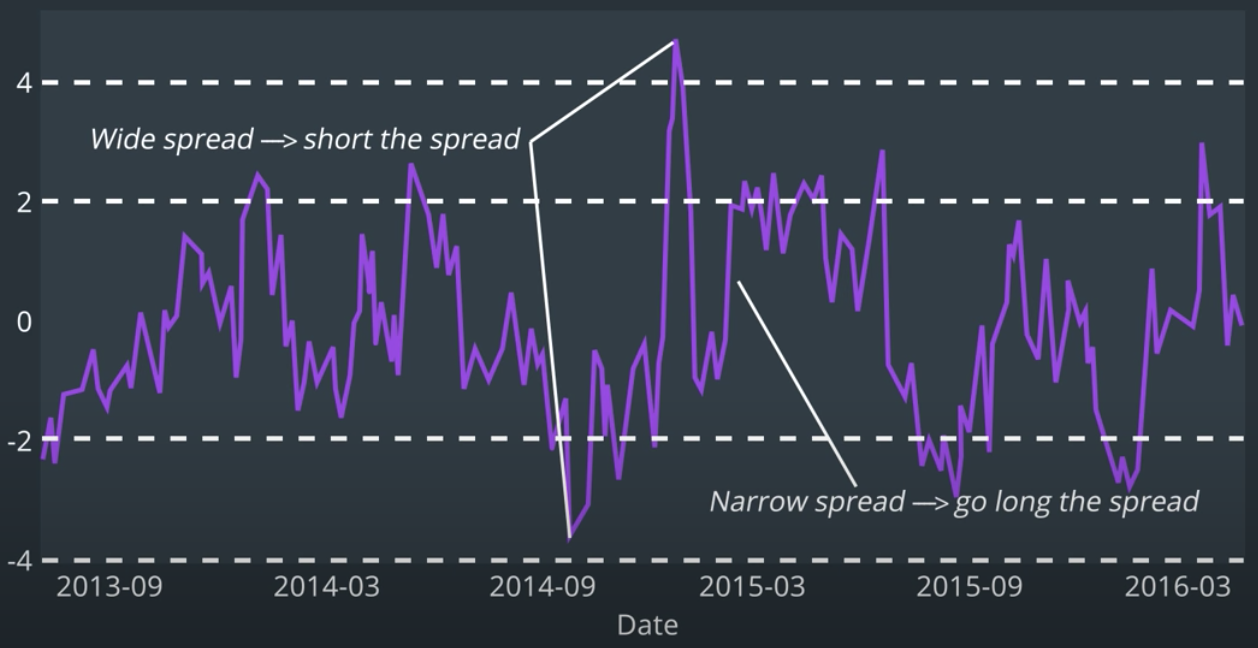
If spread widens, short the spread: short the asset that has increased, long the asset that has decreased (relatively).
If spread narrows, go long the spread: short asset that has increased, long the asset that has decreased (relatively).
-
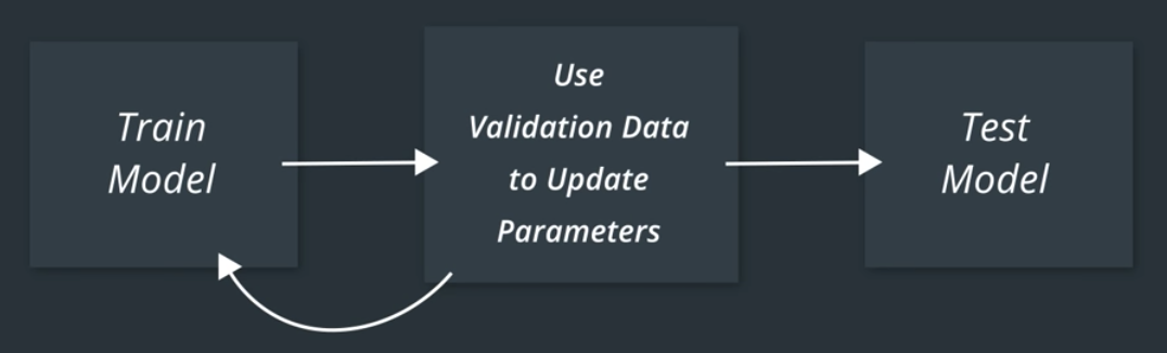
Backtest
Cointegration Test: Engle-Granger
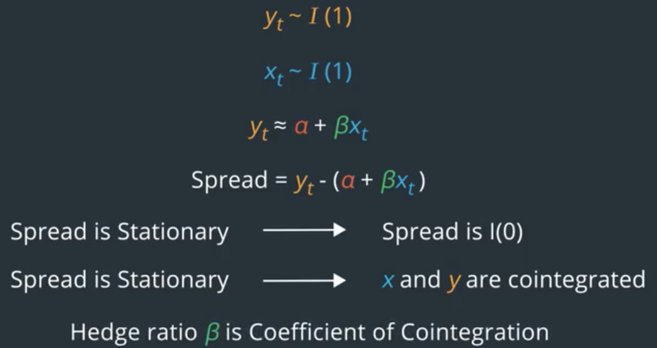
- Get hedge ratio from a linear regression
- Calculate spread and check if the spread is stationary
Implement code about the linear regression:
# s1, s2: Series

# 0      99.72323240
# 1     100.30508341
# 2     102.45348267
# 3     101.17399567
# 4     101.67627255
#           ...
# 995   126.61157374
# 996   127.49596808
# 997   126.08527093
# 998   127.17812966
# 999   128.69463841
# Name: s1, Length: 1000, dtype: float64

lr = LinearRegression()
lr.fit(s1.values.reshape(-1,1),s2.values.reshape(-1,1))

hedge_ratio = lr.coef_[0][0]
intercept = lr.intercept_[0]
Stationary Test: Augmented Dickey Fuller
To check if spread is stationary using Augmented Dickey Fuller Test
p-value < 0.05, spread is stationary, and therefore two stocks are cointegrated.
The adfuller function is part of the statsmodel library.
adfuller(x, maxlag=None, regression='c', autolag='AIC', store=False, regresults=False)[source]

adf (float) – Test statistic
pvalue (float) – p-value
Code implement:
def is_spread_stationary(spread, p_level=0.05):
    """
    spread: obtained from linear combination of two series with a hedge ratio

    p_level: level of significance required to reject null hypothesis of non-stationarity

    returns:
        True if spread can be considered stationary
        False otherwise
    """
    #TODO: use the adfuller function to check the spread
    adf_result = adfuller(spread)

    #get the p-value
    pvalue = adf_result[1]

    print(f"pvalue {pvalue:.4f}")
    if pvalue <= p_level:
        print(f"pvalue is <= {p_level}, assume spread is stationary")
        return True
    else:
        print(f"pvalue is > {p_level}, assume spread is not stationary")
        return False
Mathematical Formula
In order to test for stationarity, we need to test for something called a unit root. Autoregressive unit root test are based the following hypothesis test:
\[\begin{aligned} H_{0} & : \phi =\ 1\ \implies y_{t} \sim I(0) \ | \ (unit \ root) \\ H_{1} & : |\phi| <\ 1\ \implies y_{t} \sim I(0) \ | \ (stationary) \\ \end{aligned}\]It’s referred to as a unit root tet because under the null hypothesis, the autoregressive polynominal of $\scr{z}_{t},\ \phi (\scr{z})=\ (1-\phi \scr{z}) \ = 0$, has a root equal to unity.
$y_{t}$ is trend stationary under the null hypothesis. If $y_{t}$is then first differenced, it becomes: \(\begin{aligned} \Delta y_{t} & = \delta\ + \Delta\scr{z}_{t} \\ \Delta \scr_{z} & = \phi\Delta\scr{z}_{t-1}\ +\ \varepsilon_{t}\ -\ \varepsilon_{t-1} \\ \end{aligned}\)
The test statistic is
\[t_{\phi=1}=\frac{\hat{\phi}-1}{SE(\hat{\phi})}\]$\hat{\phi}$ is the least square estimate and SE($\hat{\phi}$) is the usual standard error estimate. The test is a one-sided left tail test. If {$y_{t}$} is stationary, then it can be shown that
\[\sqrt{T}(\hat{\phi}-\phi)\xrightarrow[\text{}]{\text{d}}N(0,(1-\phi^{2}))\]or
\[\hat{\phi}\overset{\text{A}}{\sim}N\bigg(\phi,\frac{1}{T}(1-\phi^{2}) \bigg)\]andit follows that $t_{\phi=1}\overset{\text{A}}{\sim}N(0,1).$ However, under the null hypothesis of non-stationarity, the above result gives
\[\hat{\phi}\overset{\text{A}}{\sim} N(0,1)\]The following function will allow us to check for stationarity using the Augmented Dickey Fuller (ADF) test.